
In unsupervised learning, choosing the right number of clusters can have a dramatic impact on clustering results (and their usefulness). Here, I will discuss some techniques that can be used to determine the optimal number of clusters to use in our analysis. Obviously, I am not going to consider algorithms that can determine the number automatically (like density-based algorithms, hierarchical algorithms, or GMM).
Silhouette Score
The silhouette score quantifies how well each data point fits into its assigned cluster compared to other clusters. The score ranges is defined in the interval $[-1; 1]$, a value close to 1 indicating that the cluster assignment is appropriate. The optimal number of clusters maximises the average silhouette score across all data points.
In code it can be calculated as:
from sklearn.metrics import silhouette_score

silhouette_scores = []
for i in range(2, 11):
    kmeans = KMeans(n_clusters=i, init='k-means++', random_state=42)
    kmeans.fit(data)
    score = silhouette_score(data, kmeans.labels_)
    silhouette_scores.append(score)

plt.plot(range(2, 11), silhouette_scores)
plt.title('Silhouette Score')
plt.xlabel('Number of Clusters')
plt.ylabel('Silhouette Score')
plt.show()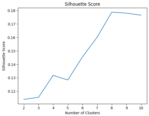
In this case the optimal number of clusters is 8, but 9 and 10 are also close to that.
The silhouette score provides an intuitive measure of cluster cohesion and separation, considering both intra-cluster similarity and inter-cluster distance. This makes it a robust metric for determining the optimal number of clusters, which has the additional benefit of being less sensitive to the shape and density of clusters compared to other methods.
Davies-Bouldin index
This index measures the average distance between each cluster’s data points and the centroid of its closest cluster. It considers both intra-cluster similarity and inter-cluster distance, with lower values indicating better clustering.
In code this calculation can be performed like this:
from sklearn.metrics import davies_bouldin_score

db_scores = []
for i in range(2, 11):
    kmeans = KMeans(n_clusters=i, init='k-means++', random_state=42)
    kmeans.fit(data)
    score = davies_bouldin_score(data, kmeans.labels_)
    db_scores.append(score)

plt.plot(range(2, 11), db_scores)
plt.title('Davies-Bouldin Index')
plt.xlabel('Number of Clusters')
plt.ylabel('Davies-Bouldin Index')
plt.show()

Similarly to the Silhouette score, the Davies-Bouldin index identifies the optimal number of cluster for the dataset (the same as above) as 8.
The Davies-Bouldin index also provides a measure of intra-cluster similarity and indication of inter-cluster distance.
Elbow Method
The elbow method involves plotting the within-cluster sum of squares (WCSS) against the number of clusters. As the number of clusters increases, the WCSS typically decreases. However, beyond a certain point, the rate of decrease slows down, resulting in an “elbow” point on the plot. This elbow point signifies the optimal number of clusters.
Working on the same dataset as the previous cases, we can apply the Elbow method as follows:
from sklearn.cluster import KMeans
import matplotlib.pyplot as plt

wcss = []
for i in range(1, 11):
    kmeans = KMeans(n_clusters=i, init='k-means++', random_state=42)
    kmeans.fit(data)
    wcss.append(kmeans.inertia_)

plt.plot(range(1, 11), wcss)
plt.title('Elbow Method')
plt.xlabel('Number of Clusters')
plt.ylabel('WCSS')
plt.show()
The graph shows the results of applying the Elbow method alongside its biggest weakness: sometimes it’s difficult to obtain definitive results out of it, and it’s best used in conjunction with some other methods.
Even though it’s not always enough, the elbow method offers a visual representation of the trade-off between the number of clusters and the within-cluster sum of squares (WCSS) and it can be helpful in some situations.
Gap statistics
Gap statistics compare the total intracluster variation for different numbers of clusters with their expected values under a null reference distribution. The optimal number of clusters is where the gap statistic is maximized. This method takes into account both the dispersion within clusters and the overall dataset’s structure.
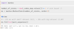
In code it can be implemented like this:
from gap_statistic import OptimalK

optimalK = OptimalK(parallel_backend='multiprocessing')
n_clusters = optimalK(data, cluster_array=np.arange(1, 11))
print(f'Optimal number of clusters: {n_clusters}')
The value returned by this method in our situation is 9, which is in line (although not perfectly) with previous analyses.
Here we compare the observed within-cluster variation with a null reference distribution, aiming to identify the optimal number of clusters where the gap statistic is maximized. This approach can provide valuable insights into cluster structure at the price of computational intensity and sensitivity to the reference distribution. These factor can have limiting effects on the usefulness of this technique in some scenarios.
Average Distance to Centroid
This technique involves calculating the average distance between each data point and its assigned cluster centroid. The optimal number of clusters corresponds to a significant decrease in the average distance, indicating tight and well-separated clusters.
It can be implemented and visualised like this:
from scipy.spatial.distance import cdistavg_distances = []
for i in range(1, 11):
kmeans = KMeans(n_clusters=i, init='k-means++', random_state=42)
kmeans.fit(data)
centroids = kmeans.cluster_centers_
avg_distance = np.mean(np.min(cdist(data, centroids, 'euclidean'), axis=1))
avg_distances.append(avg_distance)
plt.plot(range(1, 11), avg_distances)
plt.title('Average Distance to Centroid')
plt.xlabel('Number of Clusters')
plt.ylabel('Average Distance')
plt.show()
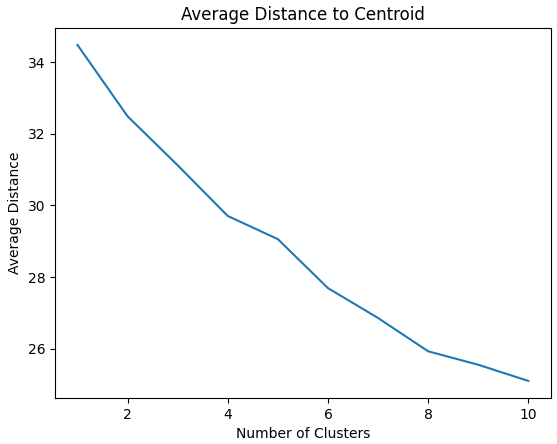
In this case the optimal number of centroids is identified to be 10, which somewhat aligns with previous techniques.
The average distance to centroid offers a straightforward approach to evaluating cluster tightness and separation, even though it may not capture the full complexity of cluster structures. This is especially true in datasets with irregular shapes or varying cluster densities. Another potential issue is that the interpretation of average distance metrics can be less intuitive compared to other techniques, and that the choice of the distance metric should depende on the dataset, its dimensionality and characteristics, and it can have a strong impact on the final result.

 order Markov Chains, whereas our problem would have been better defined by a
  order Markov Chain (more details below).
 having the property that, given the present, the future is conditionally independent of the past:


 is the transition matrix.
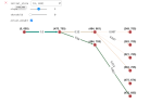
 order MC (seen in the `inital_state` box, as it contains two values).